In the first post in this series, we introduced the concept of factor investing and talked about the origin of the concept. Building upon that foundation, this article will direct our focus towards the “traditional” collection of investment factors that have remained prominent throughout the existence of this concept. The code discussed within this article will be made available via a link provided at its conclusion.
Getting Data
One of the main sources of data for the “traditional” set of risk factors is Ken French’s “Data Library” website. Ken - as you may remember from the previous post - is the co-creator of the “Fama-French Three Factor Model” alongside Eugene Fama. Ken provides a great service to the finance world by curating and offering these data for general use - his data library is used regularly by academics and practitioners alike. Ken’s site offers data in the form of text files which provide daily, or monthly returns.
In order to make the gathering of these data a bit more convenient, we will access these data via the “getFamaFrenchFactors” python module.
# Installation
pip install getFamaFrenchFactors
# Sample Usage
import getFamaFrenchFactors as gff

# Get the Fama-French three factor model (monthly data)
df_ff3_monthly = gff.famaFrench3Factor(frequency='m')

# Get the Fama-French three factor model (annual data)
df_ff3_annual = gff.famaFrench3Factor(frequency='a')
This module just provides a convenient way of capturing data from Ken’s website. In the event that you want to calculate the factor returns yourself - and if you have a WRDS account, you can use the famafrench module. But for this post we’ll just take the pre-prepared data from Ken’s website.
Fama-French Three Factor Model
To recap, the Fama-French Three Factor model aims to explain stock returns using three1 primary risk factors: market return, the “size” or “SMB” factor return, and the “value” or “HML” factor return. These factors, along with some random noise, collectively account for the fluctuations in stock returns. The model suggests that each stock’s return is influenced by a combination of these three factors to differing extents.
\[R_{i,t} - R_{f,t} = \beta_{i} \times (R_{M,t} - R_{f,t}) + s_{i} \times SMB_{t} + h_{i} \times HML_{t} + \epsilon_{i,t}\]where:
- $R_{i,t}$ is the return of asset $i$ at time $t$
- $R_{f,t}$ is the risk-free rate at time $t$
- $\beta_{i}$ is the sensitivity of asset $i$ to the market factor
- $R_{M,t}$ is the return on the market portfolio at time $t$
- $SMB_{t}$ is the return difference between small and large firms at time $t$
- $s_{i}$ is the sensitivity of asset $i$ to the SMB factor
- $HML_{t}$ is the return difference between high and low book-to-market equity firms at time $t$
- $h_{i}$ is the sensitivity of asset $i$ to the HML factor
- $\epsilon_{i,t}$ is the idiosyncratic error term.
We can get all the data for the Three Factor model by using the getFamaFrenchFactors module:
import getFamaFrenchFactors as gff
df_ff3_monthly = gff.famaFrench3Factor(frequency='m')
df_ff3_monthly.set_index('date_ff_factors', inplace=True)
Let’s see what the most recent 10 rows look like by doing df_ff3_monthly.tail(10)…
| date_ff_factors | Mkt-RF | SMB | HML | RF |
|---|---|---|---|---|
| 2022-09-30 00:00:00 | -0.0935 | -0.0079 | 0.0006 | 0.0019 |
| 2022-10-31 00:00:00 | 0.0783 | 0.0009 | 0.0805 | 0.0023 |
| 2022-11-30 00:00:00 | 0.046 | -0.034 | 0.0138 | 0.0029 |
| 2022-12-31 00:00:00 | -0.0641 | -0.0068 | 0.0132 | 0.0033 |
| 2023-01-31 00:00:00 | 0.0665 | 0.0502 | -0.0405 | 0.0035 |
| 2023-02-28 00:00:00 | -0.0258 | 0.0121 | -0.0078 | 0.0034 |
| 2023-03-31 00:00:00 | 0.0251 | -0.0559 | -0.0901 | 0.0036 |
| 2023-04-30 00:00:00 | 0.0061 | -0.0334 | -0.0003 | 0.0035 |
| 2023-05-31 00:00:00 | 0.0035 | 0.0153 | -0.078 | 0.0036 |
| 2023-06-30 00:00:00 | 0.0646 | 0.0155 | -0.002 | 0.004 |
So we have a big dataframe - each row represents the end-of-month return, and the columns in order represent…
- Mkt-RF = Market return minus Risk-Free return, often referred to as the Market Risk Premium (MRP) or the Market’s Excess Return. This figure represents the compensation for exposing your capital to risk through market investment, as opposed to the alternative of depositing funds in a bank or investing in a “safe” asset like a short-term bond2
- SMB = Small Minus Big, or the difference in returns between Small companies and Big companies
- HML = High Minus Low, or the difference in returns between companies with High valuations, and companies with Low valuations
- RF = Risk Free Rate, or the return on a “risk free” asset
Size (SMB)
Conceptual basis: Small companies tend to yield higher returns compared to large companies. Consequently, adopting a strategy of purchasing small companies while selling larger companies short should yield favourable returns. This rationale gives rise to the terminology “small minus big” or “SMB.”
Potential explanatory theories include:
- Reduced liquidity in small caps, thus resulting in a reward for taking on liquidity risk
- Smaller companies have more growth potential
- Smaller companies are more agile as they require less capital to fund a strategy change
Lets get the monthly returns for the Size factor and plot it to see visually how it looks…
# Filter on the SMB column and plot a cumulative return line chart
df_size = df_ff3_monthly['SMB']
df_size.cumsum().plot(title='SMB Factor Cumulative Returns')

# Print some performance metrics
annual_volatility = df_size.std()*(12**0.5)
mean_annualized_return = df_size.mean()*12
print(f"Cumulative Return: {round(df_size.sum()*100, 2)}%\
	\nMean Annual Return: {round(mean_annualized_return*100, 2)}%\
	\nAnnualised Volatility: {round(annual_volatility*100, 2)}%\
	\nAnnual Sharpe Ratio: {round(mean_annualized_return/annual_volatility, 2)}")
Cumulative Return: 219.53%
Mean Annual Return: 2.26%
Annualised Volatility: 10.98%
Annual Sharpe Ratio: 0.21
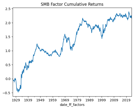
So this is some numerical and visual information on the returns of the “Size” factor. I don’t want to make you re-read the same python code so I am going to make this into a function which we will reuse several times…
def show_me_factor_info(factor, df):
	df_single_factor = df[factor]
	df_single_factor.cumsum().plot(title='{} Factor Cumulative Returns'.format(factor))
	annual_volatility = df_single_factor.std()*(12**0.5)
	mean_annualized_return = df_single_factor.mean()*12
	print(f"Cumulative Return: {round(df_single_factor.sum()*100, 2)}%\
		\nMean Annual Return: {round(mean_annualized_return*100, 2)}%\
		\nAnnualised Volatility: {round(annual_volatility*100, 2)}%\
		\nAnnual Sharpe Ratio: {round(mean_annualized_return/annual_volatility, 2)}")

# Usage Example
show_me_factor_info('SMB', df_ff3_monthly)
Value
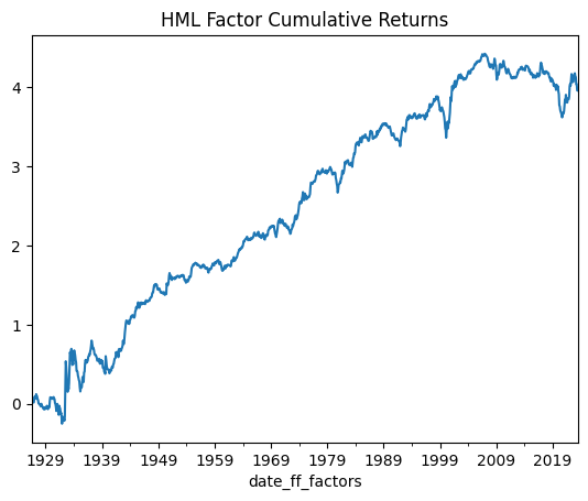
Conceptual basis: Inexpensively valued companies tend to generate higher returns than their pricier counterparts.
Potential explanatory theories include:
- This phenomenon may be attributed to companies with substantial debt or erratic earnings being undervalued.
- Investor aversion to companies that have demonstrated past underperformance.
- Such companies are likelier to revert to, or surpass, a 1-1 price-to-book ratio.
show_me_factor_info('HML', df_ff3_monthly)
Output
Cumulative Return: 395.84%
Mean Annual Return: 4.08%
Annualised Volatility: 12.38%
Annual Sharpe Ratio: 0.33
Carhart Four Factor Model
The Carhart Four Factor Model builds upon the foundation of the Fama-French Three Factor model by introducing “Momentum” as an additional explanatory factor. This expansion involves incorporating Momentum into the existing framework and was exemplified in Mark Carhart’s 2012 paper titled “On Persistence in Mutual Fund Performance.”
\[R_{i,t} - R_{f,t} = \beta_{i} \times (R_{M,t} - R_{f,t}) + s_{i} \times SMB_{t} + h_{i} \times HML_{t} + u_{i} \times UMD_{t} + \epsilon_{i,t}\]where:
- $R_{i,t}$ is the return of asset $i$ at time $t$
- $R_{f,t}$ is the risk-free rate at time $t$
- $\beta_{i}$ is the sensitivity of asset $i$ to the market factor
- $R_{M,t}$ is the return on the market portfolio at time $t$
- $s_{i}$ is the sensitivity of asset $i$ to the SMB factor
- $SMB_{t}$ is the return difference between small and large firms at time $t$
- $h_{i}$ is the sensitivity of asset $i$ to the HML factor
- $HML_{t}$ is the return difference between high and low book-to-market equity firms at time $t$
- $u_{i}$ is the sensitivity of asset $i$ to the UMD factor
- $UMD_{t}$ is the return difference between winners and losers at the time $t$
- $\epsilon_{i,t}$ is the idiosyncratic error term
If you contrast this with the preceding section, you’ll observe the addition of a new component in the equation, denoted as “UMD,” signifying Up Minus Down. This element encapsulates the returns associated with owning companies whose stock prices have risen (winners) versus the returns of companies whose stock prices have fallen (losers). This phenomenon is commonly recognized as “Momentum,” reflecting the upward or downward momentum in stock prices. The pioneering paper on Momentum is “Returns to Buying Winners and Selling Losers” authored by Jegadeesh and Titman, published in 1993.
Momentum
Underlying thinking: Companies that have performed well recently will continue to perform well in the near future
Potential explanatory theories include:
- Behavioral factors such as herding behavior and confirmation bias
- Investor tendencies towards both underreacting and overreacting
- Influence of supply and demand dynamics, including factors related to indexation
df_c4f_monthly = gff.carhart4Factor(frequency='m')
df_c4f_monthly.set_index('date_ff_factors', inplace=True)
show_me_factor_info('MOM', df_c4f_monthly)
Cumulative Return: 726.44%
Mean Annual Return: 7.53%
Annualised Volatility: 16.31%
Annual Sharpe Ratio: 0.46
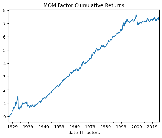
While Momentum has exhibited robust long-term performance, it’s important to acknowledge that this factor is susceptible to significant crashes. If we take a step back and examine the data, we can identify instances of these substantial downturns, notably around 1929 and 2009. It’s worth noting that on the logarithmic scale of the chart, these crashes might appear less severe than they truly were. To gain a clearer perspective, let’s reassess the chart by depicting the losses over time as a percentage of the peak value, commonly referred to as the “Max Drawdown.”
## Turn Log Returns into Simple Returns
import numpy as np
mom_simple_returns = (np.exp(df_c4f_monthly['MOM'])).fillna(1)
cumulative_reinvested_return = mom_simple_returns.cumprod()

# Plot the Max Drawdown time series
((cumulative_reinvested_return - cumulative_reinvested_return.expanding().max())/
(cumulative_reinvested_return.expanding().max())*100).plot(title='MOM Max Drawdown in %')
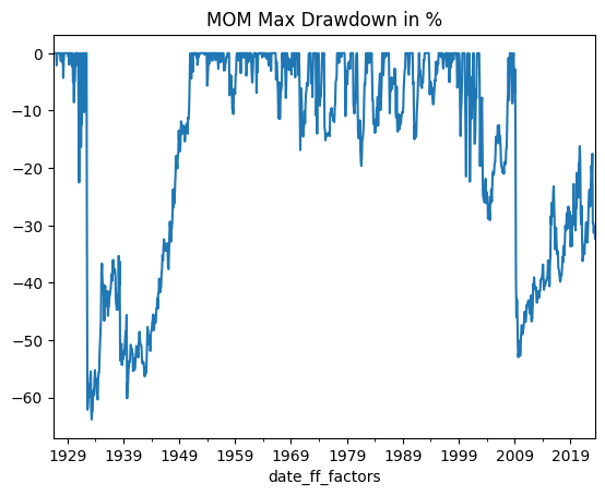
A commonly held notion suggests that a maximum drawdown of around 30% is generally considered tolerable for investors with a reasonable risk appetite. However, it’s important to acknowledge that this is largely anecdotal and lacks definitive scientific evidence—it’s more of a rule of thumb. Evaluating the max drawdowns for the Momentum factor, the period from 1950 to 2008 appears relatively manageable. In contrast, the drawdowns observed prior to and following this time frame are notably deep, with the prospect of experiencing a rapid 50% loss over a few months being particularly unpleasant. This underscores one of the principal risks inherent in Momentum investing—namely, the potential for significant crashes. Due to the operational mechanics of Momentum strategies, recovery from such crashes often demands a considerable amount of time.
Fama-French Five Factor Model
In 2015, Eugene Fama and Ken French published an extension of their Three Factor model which includes two new factors…
- Robust Minus Weak (RMB) which reflects returns on companies with strong operating profitability ratios as compared to companies with weak operating profitability ratios. This is commonly referred to as the “profitability” factor.
- Conservative Minus Aggressive (CMA) which reflects returns on companies with a conservative approach or level of investment in itself minus returns on companies with an aggressive approach or level of investment in itself. This is commonly referred to as the “growth” or “capex” factor
So now we have to update our arithmetic again to account for the two new explanatory factors…
\[R_{i,t} - R_{f,t} = \beta_{i}(R_{M,t} - R_{f,t}) + s_{i}SMB_{t} + h_{i}HML_{t} + p_iRMW_{t} + g_iCMA_{t} + \epsilon_{i,t}\]where:
- $R_{i,t}$ is the return of asset $i$ at time $t$.
- $R_{f,t}$ is the risk-free rate at time $t$.
- $\beta_{i}$ is the sensitivity of asset $i$ to the market factor.
- $R_{M,t}$ is the return on the market portfolio at time $t$.
- $s_{i}$ is the sensitivity of asset $i$ to the SMB factor.
- $SMB_{t}$ is the return difference between small and large firms at time $t$.
- $h_{i}$ is the sensitivity of asset $i$ to the HML factor.
- $HML_{t}$ is the return difference between high and low book-to-market equity firms at time $t$.
- $p_{i}$ is the sensitivity of asset $i$ to the RMW factor.
- $RMW_{t}$ is the return difference between high and low profitability firms at the time $t$.
- $g_{i}$ is the sensitivity of asset $i$ to the CMA factor.
- $CMA_{t}$ is the return difference between high and low growth firms at the time $t$.
- $\epsilon_{i,t}$ is the idiosyncratic error term.
Although the addition of these two factors filled some gaps in the literature, some academics and practitioners had mixed views on the efficacy of the Five Factor model. Robeco - a large institutional asset manager specialising in factor-based investing, among other approaches - noted surprise that Momentum was not formally included as a factor, leaving it to be covered by Carhart’s model, especially given that it had so much explanatory power. Others noted that the existence of the Low Volatility factor (a non-traditional factor which will be explored in a later post) which directly contradicts the existing Market Risk Premium factor present in both the three and five factor models has not been dealt with. Nevertheless, despite these critiques, the Five Factor model’s incorporation of the “Profitability” and “Investment” factors represented an enhancement over the original Three Factor model, even in light of its inherent limitations.
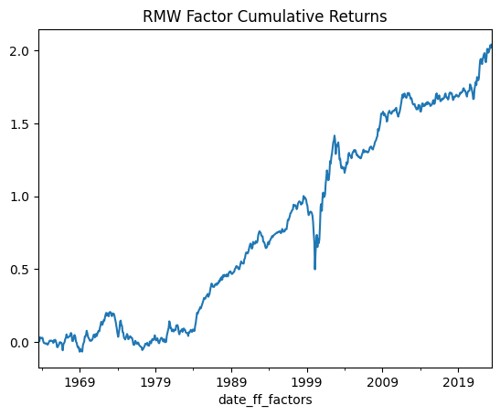
Profitability
Suggestion: Companies with higher profit margins earn higher returns than those with lower profit margins
Potential explanatory theories include:
- Profitable firms tend to be growth firms and thus are likely to appreciate in value
- Profitable companies might be less volatile and thus not popular for “prospecting”
- Profitable firms are less prone to distress
df_ff5f_monthly = gff.famaFrench5Factor(frequency='m')
df_ff5f_monthly.set_index('date_ff_factors', inplace=True)
show_me_factor_info('RMW', df_ff5f_monthly)
Cumulative Return: 204.1%
Mean Annual Return: 3.4%
Annualised Volatility: 7.69%
Annual Sharpe Ratio: 0.44
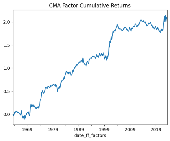
Investment
Suggestion: Companies who are re-investing a lot earn higher returns than those are a not
Potential explanatory theories include:
- Reinvestment and CAPEX signal future growth of the company
- Reinvestment and CAPEX signal market opportunities which have yet to be captured
show_me_factor_info('CMA', df_ff5f_monthly)
Cumulative Return: 200.32%
Mean Annual Return: 3.34%
Annualised Volatility: 7.21%
Annual Sharpe Ratio: 0.46
At this point, you might notice something interesting. Both the Profitability and Investment factors perform well during times of market stress. Let’s plot them beside the general Market return and zoom in on the 1999 to 2022 period…
title = 'CMA/RMW Returns vs. Market Returns 1999 to 2022'
df_ff5f_monthly[['CMA', 'RMW', 'Mkt-RF']].loc['1999':'2022'].cumsum().plot(title=title)
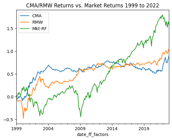
Visually we can see that during the Dot com bubble and poor performance thereafter (2000 to 2003) the market performed poorly whereas RMW and CMA did quite well. Likewise we see a similar trend in 2007 to 2009 and 2022. We can see that the correlations of monthly returns for RMW and CMA against the Market return for this slice of time are negative at -0.35 and -0.26 respectively…
df_ff5f_monthly[['CMA', 'RMW', 'Mkt-RF']].loc['1999':'2022'].corr()
| CMA | RMW | Mkt-RF | |
|---|---|---|---|
| CMA | 1 | 0.252842 | -0.264515 |
| RMW | 0.252842 | 1 | -0.349071 |
| Mkt-RF | -0.264515 | -0.349071 | 1 |
Behaviourally we could come up with some explanations for this…
- 2000 to 2003: internet stocks with weak (or no) earnings and lots of aggressive capex are sold off and tank in value. RMW and CMA factors would perform well as they capture returns for companies with strong earnings and conservative capital expenditure
- 2007 to 2009: the credit crunch causes a “flight to quality” - investors reallocate funds to safer companies to mitigate risk
- 2022: interest rates rise causing funding challenges for high growth companies, resulting in losses for tech stocks, echoing the 2000 to 2003 period.
What’s next?
In the next post, we’ll look at various approaches to performing factor regressions, which should illustrate the reason why these factors are so useful in explaining the sources or drivers of returns for investors. In the post after that, we’ll look at some “non-traditional” investment factors and talk about how to make sense of the “Factor Zoo”.
The code for this post is available on github here.
-
Technically four factors if you include the Risk Free Rate as a “factor”. It’s certainly time-varying but in general its not included as a risk factor because there’s no variation in how much the risk free rate impacts each stock. In more technical terms, market, size and value factors are factors because their coefficients vary in the cross-section of returns, whereas the risk free rate’s coefficient is always 1. ↩
-
In general the Risk Free return is either the Effective Federal Funds Rate or some similar short duration deposit facility. In past experience I’ve seen people use the US 10 Year Treasury Bond Yield as a risk-free rate, but that is by no means risk free. In general a risk-free rate could be defined differently for each investor based on what investments they have access to, their holding period, their geographic location, and other such factors. ↩