Measuring Factor Exposure

In the first installment of this series, we introduced the concept of risk factors in the realm of finance and investing, and explored their historical backgrounds. In the second post, we examined the specific “traditional” factor exposures—such as Size and Value—individually, illustrating their return patterns. In this article, our focus will shift towards understanding how to quantify a stock’s or a portfolio’s exposure to these factors. Additionally, we’ll explain some of the reasons motivating such measurements, both in personal and professional contexts.

Why factor exposure might be important to you

Let’s say for example that you’re a hedge fund manager who employs traders or portfolio managers with superior stock picking skill, and whose returns have low - or no - correlation with the market. Furthermore, you may say to yourself “not only do I want returns which are materially different or uncorrelated to the market, I also want their returns to be uncorrelated to the well known risk premiums like Momentum”. Factors are essentially risk premiums, and risk premiums hypothesise that if you take a certain risk, you should get a certain compensation for it. And as a hedge fund manager, you’re not compensating these people in return for just getting you exposure to well-known returns! You want returns which are not explainable by the market’s returns or the well known risk premiums, and this “un-explainable” return is often referred to as “alpha”.

Now, let’s think about the opposite perspective of someone who might want to prove that they are exposed to these factors. Imagine you work for an asset manager that issues and oversees a myriad of exchange-traded funds and mutual funds, all designed to mimic the returns closely aligned with factors like Value, Size, Momentum. Your clients might use your funds to diversify their holdings or perhaps because they see tactical opportunities to “time” their exposure to a specific factor. Imagine that someone raises concerns about one of your funds—the “US Value ETF.” They’re worried that it’s “beta” exposure to the Value factor hypothetical returns are not sufficiently significant. This can be due to a poorly specified investment approach, or some other effect such as style drift. This situation will likely prompt you t o seek out multiple avenues—both qualitative and quantitative—to validate that your fund is replicating Value returns as intended.

In both these scenarios, you might perform a factor regression to determine whether or not the returns of a portfolio or stock have significant exposure to one or more risk factors.

There are - of course - other reasons, such as wanting to control our risk exposure in general for risk management purposes. But let’s play with these two scenarios for now.

What are we measuring?

Although the two scenarios above explain why we might want to measure factor exposure, we haven’t been precise on what we’re measuring yet. Let’s quickly revisit the Fama French Three Factor model’s arithmetic…

\[R_{i,t} - R_{f,t} = \beta_{i} \times (R_{M,t} - R_{f,t}) + s_{i} \times SMB_{t} + h_{i} \times HML_{t} + \epsilon_{i,t}\]

where:

$R_{i,t}$ is the return of asset $i$ at time $t$
$R_{f,t}$ is the risk-free rate at time $t$
$\beta_{i}$ is the sensitivity of asset $i$ to the market factor
$R_{M,t}$ is the return on the market portfolio at time $t$
$SMB_{t}$ is the return difference between small and large firms at time $t$
$s_{i}$ is the sensitivity of asset $i$ to the SMB factor
$HML_{t}$ is the return difference between high and low book-to-market equity firms at time $t$
$h_{i}$ is the sensitivity of asset $i$ to the HML factor
$\epsilon_{i,t}$ is the idiosyncratic error term

In general, this model is asserting that it can explain all asset price returns. It’s saying that all returns ($R_{i,t} - R_{f,t}$) are made up of some amount ($\beta_{i}$) of market return ($R_{M,t} - R_{f,t}$), some amount ($s_{i}$) of Size return ($SMB_{t}$), and some amount ($h_{i}$) of Value return ($HML_{t}$), plus some random variation ($\epsilon_{i,t}$) that can be positive or negative but that averages out to be zero in the long run. But that contradicts what our hedge fund manager wants, which is returns which are not-explainable by a model like this. We can add a term called “alpha” into the model to reflect this…

\[R_{i,t} - R_{f,t} = \alpha_{i} + \beta_{i} \times (R_{M,t} - R_{f,t}) + s_{i} \times SMB_{t} + h_{i} \times HML_{t} + \epsilon_{i,t}\]

where:

$\alpha_{t}$ is the return that is not explainable by the model
everything else is the same as before

The alpha ($\alpha_{t}$) term that we just added is going to measure returns that are not explainable by this model. The Three Factor model kind of always had this term, but given that the model claims to be able to explain all returns, the model claims that the value of $\alpha$ is zero, so it is simply not shown. So the task for the hedge fund manager is to measure their trader’s alpha $\alpha$ and make sure that it ISN’T zero. If it turns out to be zero, or some number that’s not significantly different to zero, then all their returns are explained by the Three Factor model and they should be fired. In short - they will want to validate that their trader/PM has positive and significant alpha.

Our asset manager will want to measure a different thing. They will want to make sure that their returns do indeed have some amount of factor exposure. In our example, they will want to make sure that their returns are comprised of some amount ($h_{i}$) of the Value factor ($HML_{t}$). They will also want to make sure that the exposure coefficient to Value is statistically significant - it’s not good enough for their returns to be sort of exposed to the Value factor - we have to show that it has a statistically significant exposure. In short - they will want to validate that their fund has positive and significant beta to the Value factor.

We will use Ordinary Least Squares regressions to measure these values. There are more rigorous ways to specify and explain tests, but I’ll save it for another statistics-focused post which will have a bit more mathematical rigour.

Factor Regressions

To perform a factor regression, we need factor return data, and stock or portfolio data. Let’s start with some really simple examples and some boilerplate python code to gather data for stocks & etfs, as well as some Factor returns data from Ken French’s data library…

# Get the monthly log-returns for a given ticker from Yahoo Finance
def get_stock_log_returns(ticker):
data = yf.download(ticker, interval='1d', progress=False)['Close']
data = data.resample('1m').last().iloc[:-1]
log_returns = np.log(data.pct_change()+1).dropna()
log_returns.name = ticker
return log_returns

# Get the monthly log-returns from Ken French's Data Library
def get_ff_data(data, start='1-1-1960'):
factor_data = pdr.get_data_famafrench(data, start)[0]
factor_data.index = (factor_data.index.to_timestamp() + MonthEnd(0)).date
factor_data.index = pd.to_datetime(factor_data.index)
return factor_data

# Align & merge the Yahoo Finance and Factor returns dataframes
def merge_stock_and_ff_data(stock_log_rets, factor_data):
return pd.concat([stock_log_rets*100, factor_data], axis=1).dropna()

# Do all the steps above in one go
def gather_stock_factor_data(ticker='AAPL', factor_data='F-F_Research_Data_5_Factors_2x3'):
stock_data = get_stock_log_returns(ticker)
ff_data = get_ff_data(factor_data)
merged_data = merge_stock_and_ff_data(stock_data, ff_data)
return merged_data

So for example if I run gather_stock_factor_data('AMZN') I will get a dataframe that looks like this…

	AMZN	Mkt-RF	SMB	HML	RMW	CMA	RF
2023-02-28	-9.03	-2.58	0.69	-0.78	0.9	-1.4	0.34
2023-03-31	9.18	2.51	-7.01	-9.01	1.92	-2.29	0.36
2023-04-30	2.07	0.61	-2.56	-0.03	2.31	2.85	0.35
2023-05-31	13.41	0.35	-0.43	-7.8	-1.76	-7.2	0.36
2023-06-30	7.8	6.46	1.33	-0.2	2.2	-1.75	0.4

So I have data on a stock - Amazon (AMZN), and the Factor returns for the same periods in the other columns. I now need to perform an Ordinary Least Squares regression to measure the beta coefficients for each of the risk factors, and the alpha term that we talked about in the previous section. We can do this in python using Statsmodels and the following function…

def point_in_time_regression(ticker, start_date='1960-01',
        end_date=datetime.datetime.now().date()):
 merged_data = gather_stock_factor_data(ticker)
 merged_data = merged_data.loc[start_date:end_date]
 endog = merged_data[ticker] - merged_data.RF.values
 exog_vars = [item for item in list(merged_data.columns) if item not in [ticker, 'RF']]
 exog = sm.add_constant(merged_data[exog_vars])
   
 ff_model = sm.OLS(endog, exog, ).fit()
 ff_model = ff_model.get_robustcov_results(cov_type='HAC', maxlags=1)
   
 print(ff_model.summary())
   
 # Plot Partial Regression Plot:
 fig = sm.graphics.plot_partregress_grid(ff_model, fig = plt.figure(figsize=(12,8)))
 plt.show()

Let’s test it out on AAPL using the Three Factor model, and using data starting in the year 2005 and see what we get…

point_in_time_regression(
 ticker='AAPL', 
 factor_data='F-F_Research_Data_Factors', 
 start_date='2005'
)

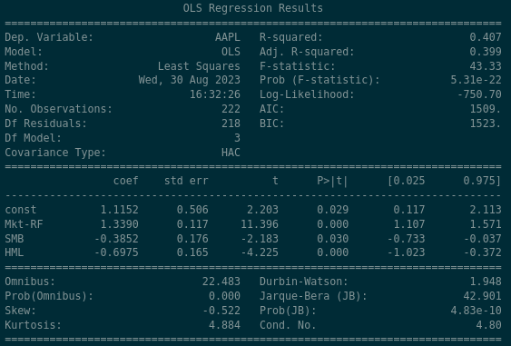
There are a lot of figures here but the important ones are listed in the middle panel here…

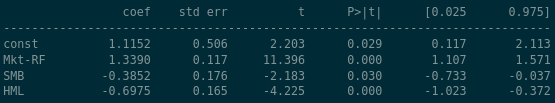
The rows of this panel are the explanatory variables that we discussed previously. “const” is short for “constant” which is another way of referring to the $\alpha$ term that we spoke about earlier. Mkt-RF, SMB, HML have also been explained earlier in this post. The values in the columns merit a little more explanation…

coef: short for coefficient, also known as the “beta” coefficient for the given variable. This is the proportion of how much of each of the explanatory variable affects the return. For example in this case the panel shows that the contribution of the Market Excess Return (Mkt-RF) is 1.3390 times its normal value
std err: short for standard error, represents a 1-standard deviation variation of the coefficient value. For example the panel says that the Market Excess Return (Mkt-RF) coefficient is 1.3390 and it varies around that number by 0.117 (so typically between 1.222 and 1.456)
t: short for t-statistic, or test statistic
P > |t|: short for p-value
[0.025 - 0.975]: The values we can observe within these percentiles of the data

So plugging these values into our Three Factor model… this regression claims the following…

\[R_{AAPL,t} - R_{f,t} = \alpha_{AAPL} + \beta_{AAPL} \times (R_{M,t} - R_{f,t}) + s_{AAPL} \times SMB_{t} + h_{AAPL} \times HML_{t} + \epsilon_{AAPL,t}\] \[R_{AAPL, t} - R_{f, t} = 1.1152 + 1.3390 \times (R_{M,t} - R_{f,t}) -0.3852 \times SMB_{t} - 0.6975 \times HML_{t} + \epsilon_{i,t}\]

Some high level statements we can draw from the regression are…

AAPL shows a positive alpha of 1.1152 which is statistically significant at the 5% level
AAPL’s “beta” to the market is approximately 1.339
AAPL has a negative relationship to the Size factor which is statistically significant at the 5% level - in other words, we expect AAPL to have a negative return when the Size factor is having positive returns. This makes sense as the Size factor reflects positive returns from owning small companies, and Apple is a huge company.
AAPL has a negative relationship to the Value factor which is significant at both the 5% and 1% levels - in other words, we expect AAPL to have negative returns when the Value factor is having positive returns. This makes sense as the Value factor reflects positive returns from owning companies with High book-to-market ratios, and Apple’s book-to-market ratio is tiny.
To summarise, AAPL moves 1.339 times as much as the market does, and has negative exposure to both the Size and Value factors.

From what we know about Apple, that was probably expected. Let’s see how Berkshire Hathaway - Warren Buffett’s value-investing focused company - looks…

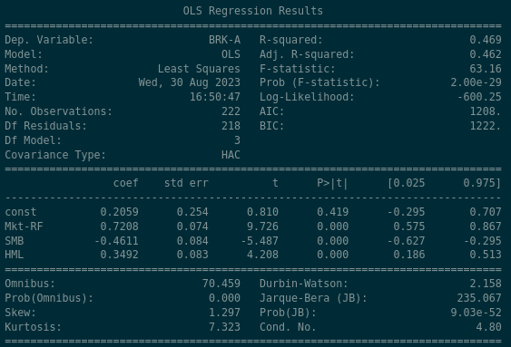
Some high level statements about Berkshire Hathaway might be…

BRK-A shows a positive alpha of 0.2059 but its not statistically significant - the value in the P > |t| column implies that there is a 41.9% likelihood that the alpha value of 0.2059 occurred by chance
BRK-A’s “beta” to the market is 0.72, so it moves less than the market does, relatively
BRK-A has a very strong negative exposure (-0.46) to the Size Factor; like Apple, Berkshire Hathway is a huge company so this is to be expected
BRK-A has a very strong positive exposure (0.34) to the Value factor, which makes sense as they are commonly known as being owners of companies with high book-to-market ratios

Back to the Scenario

At the beginning of the article, we outlined a hypothetical scenario in which we as an asset manager were getting concerning feedback that our “US Value ETF” wasn’t tracking the Value factor performance sufficiently well. We could use what we’ve learned above to examine our own fund’s exposure to the Value Factor. Let’s look at the “baseline” which might be the S&P 500 index…

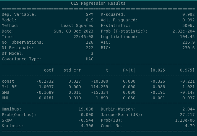
The S&P 500 index has a 0.0181 beta coefficient to the “value” factor, and the P>|t| value implies that there’s a 6% likelyhood that this is purely by chance. So with this in mind as a “baseline”, let’s look at what we see when we examine the Blackrock’s MSCI USA Value ETF…

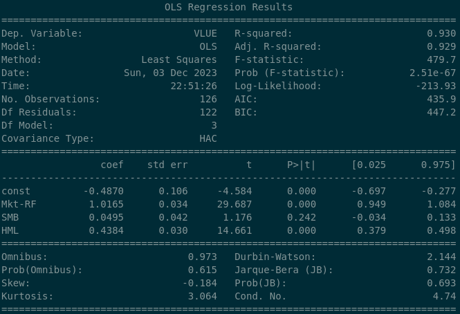
So here we can see that the Value factor exposure is dramatically different to the S&P 500 index - we see a beta coefficient of 0.4384 and which is strongly statistically significant. So over the long run we can safely say that this ETF exposes its owners to the Value factor (which we want). We can go further and do a full sample dot plot on each of the regressors…

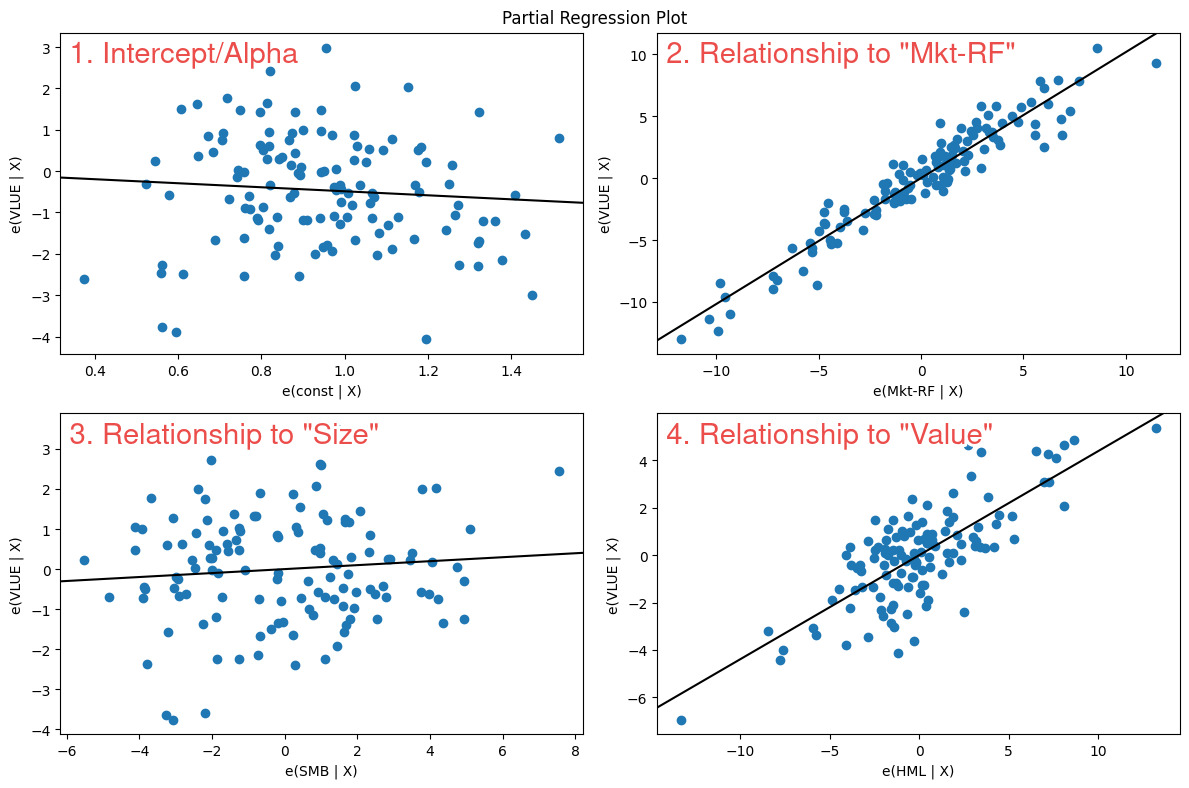
In the bottom right panel numbered #4 we can see that the line drawn through the scatter plot points upwards from left to right (positive relationship) and has an angle (slope) that moves upwards significantly. This is what we would want to see if we wanted to prove that our fund as positive & significant exposure to a factor or regressor.

Time-Series Factor Regressions

We may want to get an idea however as to how this beta or exposure varies through time. We can see that the 25th percentile exposure during the period was 0.379 and the 75th percentile exposure was 0.498. That might be nice to see in the table but I always like to see things visually if possible. Let’s write some code that will plot graphs of the rolling 5-year beta coefficients to each of our regressors (one of which is Value) over time…

def rolling_regression(ticker, window=60, factor_data='F-F_Research_Data_5_Factors_2x3', 
        start_date='1960-01', end_date=datetime.datetime.now().date()):
 merged_data = gather_stock_factor_data(ticker,factor_data=factor_data)
 merged_data = merged_data.loc[start_date:end_date]
 endog = merged_data[ticker] - merged_data.RF.values
 exog_vars = [item for item in list(merged_data.columns) if item not in [ticker, 'RF']]
 exog = sm.add_constant(merged_data[exog_vars])
 rols = RollingOLS(endog, exog, window=window)
 rres = rols.fit()
   
 print('Most recent (ending) Beta Coefficients\n\n',rres.params.iloc[-1])
 fig = rres.plot_recursive_coefficient(variables=exog_vars, figsize=(10,18))

So if we run this on ‘VLUE’ we will get the following…

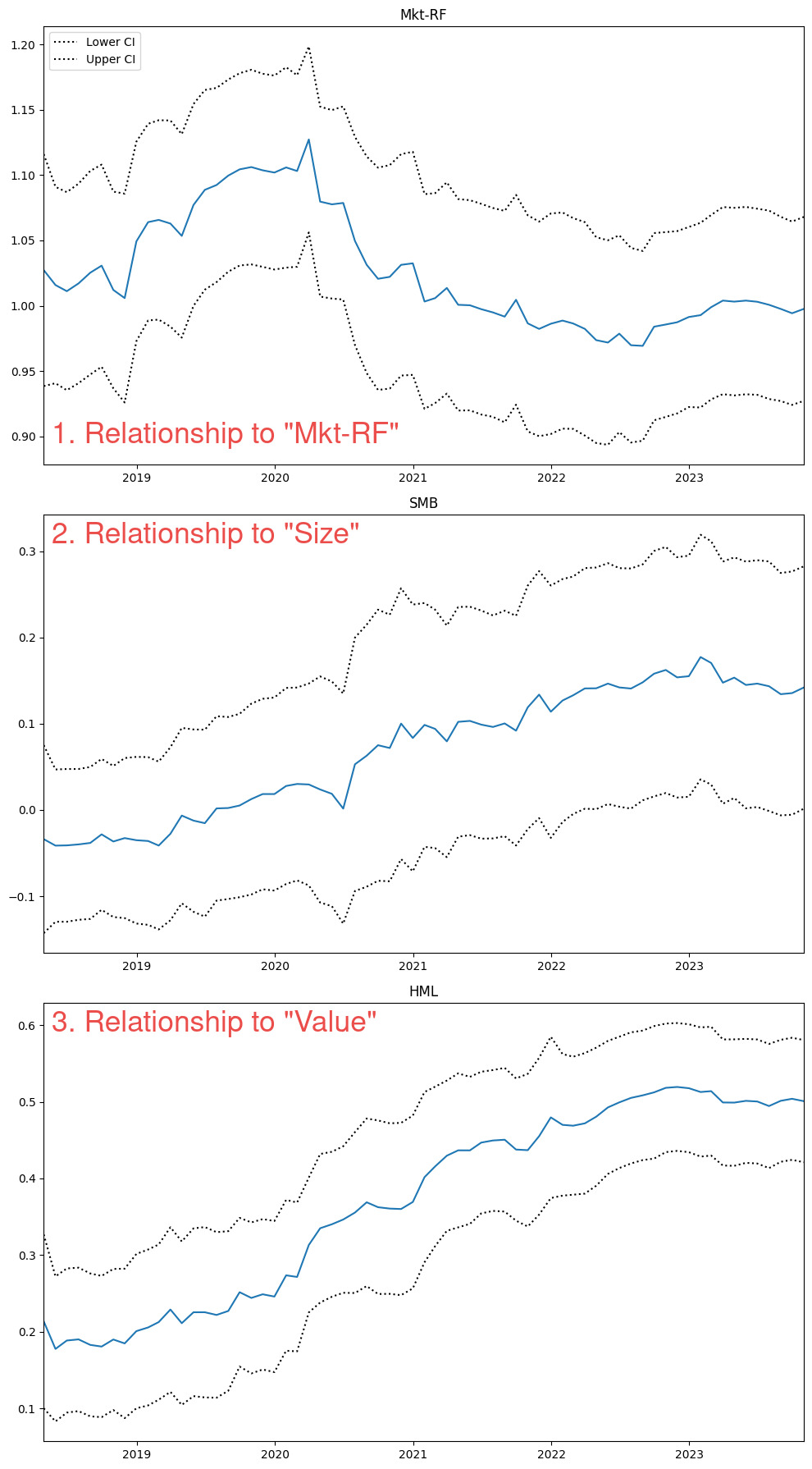
So interestingly we can see that over this period of time, the 5-year beta to “Value” increased from 0.2 in 2018 to 0.5 in 2023. A longer lookback might give some context as to why this might have occurred, but for now we should be satisfied to see these data in a time series format.

Conclusion

So now that we’ve learned how to measure factor exposure, we can confirm that our randomly picked ETF - VLUE - does indeed have exposure to the Value factor. Our hypothetical scenario is only one trivial example of how we might make use of factor regressions in the real world. We can use the practice to validate, or reject, the idea that a fund or investment strategy has exposure to a traditional risk factor. In some other cases, we might be performing this analysis expecting (or hoping) the exposure to be small and insignificant, which might imply that our investment outcomes are distinct and separate from other risk factors.

The code for this post is available on github here.